Simulation stuff
To generate (univariate) skewed data, we can use Fleishman's (1978) Power Transformation
a,b,c,dare the coefficients needed to transform the unit normal variable to a non-normal variable. NOTE:a=-c
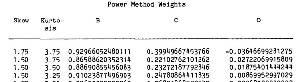
If we want a variable with a skewness of 1.75 and kurtosis of 3.75, get the coefficients from the table (p. 524)
Fleishman AI (1978). A Method for Simulating Non-normal Distributions. Psychometrika, 43, 521-532. doi: 10.1007/BF02293811
Simulation stuff
Example:
SKEWNESS KURTOSIS b c d1.75 3.75 .9297 .3995 -.0365set.seed(123)Z <- rnorm(1000)Y <- -.3995 + .9297 * Z + .3995 * Z^2 + -.0365 * Z^3hist(Y)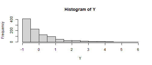
psych::skew(Y)[1] 1.765537SKEWNESS KURTOSIS b c d.75 .80 .978350485 .124833577 .001976943set.seed(123)Z <- rnorm(1000)Y <- -.12 + .98 * Z + .12 * Z^2 + .002 * Z^3hist(Y)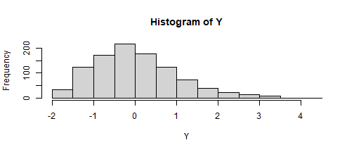
psych::skew(Y)[1] 0.7523391Simulation stuff
find_constants(method = "Fleishman", skews = 2, skurts = 10)$constants c0 c1 c2 c3 -0.20345030 0.63044307 0.20345030 0.09874172 $valid[1] "TRUE"Z <- rnorm(10000)Y <- -.20 + .63 * Z + .20 * Z^2 + .098 * Z^3hist(Y)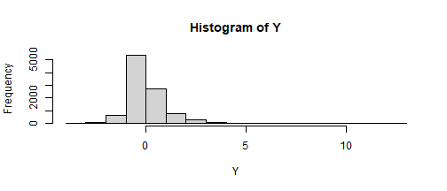
psych::skew(Y)[1] 1.947779Simulation stuff
update: Another way (not for multivariate data)-- just learned this while putting the slides together
coeff <- miceadds::fleishman_coef(mean = 0, sd = 1, skew = 2, kurt = 10)print(coeff) a b c d -0.20337308 0.63080518 0.20337308 0.09875006X1 <- miceadds::fleishman_sim(N = 10000, coef = coeff)#or... in one step...X2 <- miceadds::fleishman_sim(N = 10000, mean = 0, sd = 1, skew = 2, kurt = 10)par(mfrow = c(1, 2)) #for multipanel plot using base Rhist(X1)hist(X2)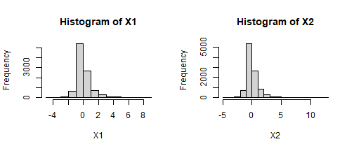
Simulation stuff
To generate multivariate, non-normal data, cannot just use the Fleishman transformation on its own (need Vale & Maurelli's method)
- Need to create an "intermediate" correlation matrix, then that is what is factor analyzed to get the transformation matrix, then the generated data is then transformed using the usual Fleishman coefficients (so there is an extra step). Again, we can just use a function to simplify this:
set.seed(234); par(mfrow = c(1, 1)) #resetting to 1 plotx2 <- mnonr::unonr(1000, c(1, 2), matrix(c(10, 2, 2, 5), 2, 2), skewness = c(-1, 2), kurtosis = c(3, 8))psych::pairs.panels(x2)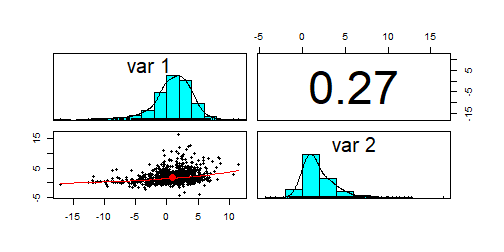
Vale, C. D. & Maurelli, V. A. (1983) Simulating multivariate non-normal distributions. Psychometrika, 48, 465-471.
Simulation stuff
Another way using the SimDesign package
library(SimDesign)set.seed(122)# univariate with skewnonnormal <- rValeMaurelli(1000, mean=10, sigma=5, skew=2, kurt=6)hist(nonnormal)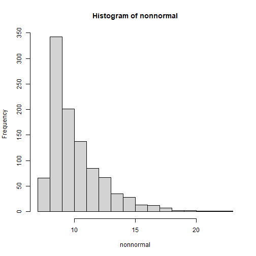
Simulation stuff
Another way using SimDesign package (cont.)
set.seed(123)n <- 10000r12 <- .4; r13 <- .9; r23 <- .1cor <- matrix(c(1,r12,r13, r12,1,r23, r13,r23,1),3,3)sk <- c(1.5,-1.5,0.5)ku <- c(3.75,3.5,0.5)nonnormal <- rValeMaurelli(n, sigma = cor, skew = sk, kurt = ku)hist(nonnormal[,1])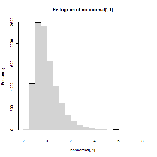
hist(nonnormal[,2])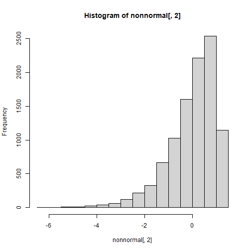
hist(nonnormal[,3])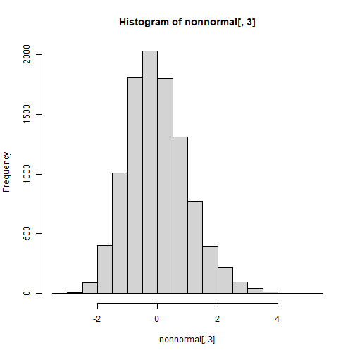
Simulation stuff
Others...
Another 'newish' package for generating simulated data is the faux (deBruine) package
- It looks interesting and has nice documentation
![]()