This is our population... we are in control of this-- we know ("theta") \(\theta\) = true value
mean(popiq)[1] 105.0702sd(popiq)[1] 14.99542hist(popiq)abline(v = mean(popiq), col = 'red')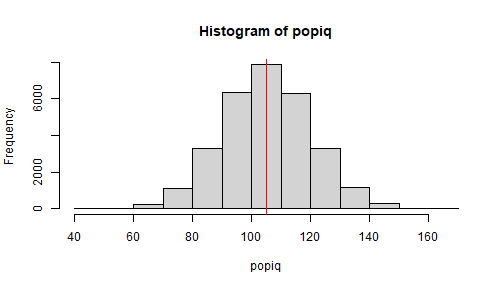
Now an important part of what we do is make inferences from a sample \(\rightarrow\) population
- We want to generalize from our sample to the population
- H0: Ability \(=\) 100
- H1: Ability \(\ne\) 100 (can also be one-tailed)
- How big a sample do we need to show this? (one sample t-test)
 Source: Wikipedia
What if we take 1000 samples of 20-- what would the distribution look like?
reps <- 1000n20 <- numeric(reps)set.seed(123)for (i in 1:reps){ n20[i] <- mean(sample(popiq, size = 20))}mean(n20)[1] 105.0358sd(n20) ## what does this represent?[1] 3.32792Although many times, our sample mean is higher than 100, there are also many occasions, due to sampling variation, where the mean is LESS than 100
hist(n20)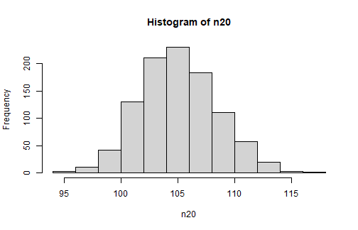
Compare distribution of means
hist(n20, xlim = c(95, 115))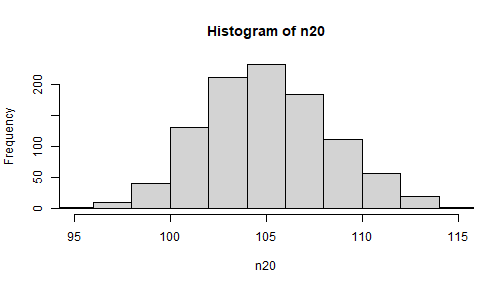
hist(n50, xlim = c(95, 115))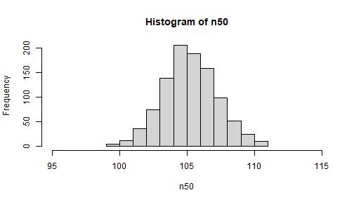
NOTE: the xlim option is specified so that the x-axes are the same in both (will not just use the default min and max which differ)
Compare distribution of means
hist(n20, xlim = c(95, 115))
hist(n50, xlim = c(95, 115))
NOTE: the xlim option is specified so that the x-axes are the same in both (will not just use the default min and max which differ)
- Many times, people think how accurate your estimate is depends on what percent of the population you sample (e.g., 10%, 50%)
- NOTE: the validity of the point estimate does not depend on the % sampled from the population-- we only have 50 out of 30,000 individuals w/c is < 1%.
What if our population did not have a normal distribution? What would the sampling distribution of means look like? \(\chi^2\) distribution
set.seed(111)skewpop <- rchisq(30000, df = 1)## mean = df; var = 2dfmean(skewpop)[1] 1.002644var(skewpop)[1] 2.021265sd(skewpop)[1] 1.421712hist(skewpop)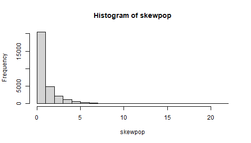
Uniform distribution (all values are equally likely) is also common...
unipop <- runif(10000, 65, 135)# var = (b - a)^2 / 12; # mean = (a + b) /2mean(unipop)[1] 100.3927(65 + 135) / 2[1] 100var(unipop)[1] 403.724(135 - 65)^2 / 12[1] 408.3333sd(unipop)[1] 20.09288hist(unipop)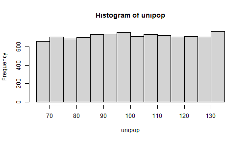 NOTE:
NOTE: runif(1000) will generated values from 0 to 1 by default.
Using the faux package... transform uni to \(\mathcal{N}\)
xnorm <- faux::unif2norm(unipop)hist(xnorm)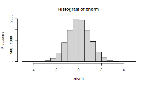
The faux packages has many functions to transform distributions. You can view the code as well how this is done.
Catan board game example...
- Rolling for resources:

Source: https://www.boardgameanalysis.com/what-is-a-balanced-catan-board/

Examine frequencies and plot this out
sjmisc::frq(rolls)x <numeric> # total N=1000 valid N=1000 mean=6.96 sd=2.46Value | N | Raw % | Valid % | Cum. %-------------------------------------- 2 | 35 | 3.50 | 3.50 | 3.50 3 | 62 | 6.20 | 6.20 | 9.70 4 | 87 | 8.70 | 8.70 | 18.40 5 | 101 | 10.10 | 10.10 | 28.50 6 | 138 | 13.80 | 13.80 | 42.30 7 | 154 | 15.40 | 15.40 | 57.70 8 | 131 | 13.10 | 13.10 | 70.80 9 | 123 | 12.30 | 12.30 | 83.10 10 | 96 | 9.60 | 9.60 | 92.70 11 | 49 | 4.90 | 4.90 | 97.60 12 | 24 | 2.40 | 2.40 | 100.00 <NA> | 0 | 0.00 | <NA> | <NA>barplot(table(rolls))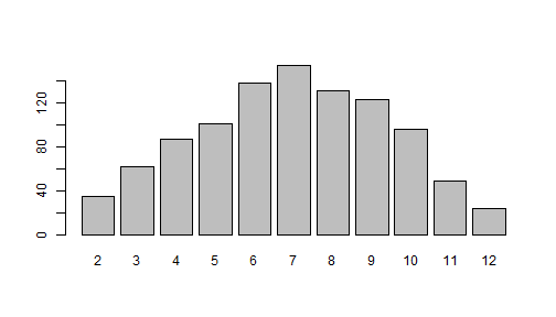 Many ways to roll a 7:
- 6-1 / 1-6
- 3-4 / 4-3
- 5-2 / 2-5
This is probably a good place to talk about functions in R...
- Things that do something in R are functions:
functionname() - This is just an example of a function with no options available
roller <- function(){ d1 <- sample(1:6, 1) d2 <- sample(1:6, 1) d1 + d2}#run the functionroller() #it works![1] 3roller()[1] 8When you run it, need the (). If not, you will just see the code.
Can use the function 1,000 times
out <- replicate(1000, roller())str(out) int [1:1000] 9 4 9 8 8 11 5 5 7 8 ...barplot(table(out)) Get the same results!
Simulation basics: Monty Hall Revisited
- As mentioned, recently reminded about this by the feature article in Chance magazine

Marilyn vos Savant, in her weekly “Ask Marilyn” column in Parade magazine, answered a reader’s question about a game show very similar to “Let’s Make a Deal”:
“Dear Marilyn: Suppose you’re on a game show, and you’re given the choice of three doors. Behind one door is a car, the others, goats. You pick a door, say number 1, and the host, who knows what’s behind the doors, opens another door, say number 3, which has a goat. He says to you, ‘Do you want to pick door number two?’ Is it to your advantage to switch your choice of doors?” –Craig F. Whitaker.
Source: https://chance.amstat.org/2022/11/monty-hall/. On another note, she was born in St. Louis, MO in 1946.
A lot has been written about this (even book/s on the topic):

At first glance, the solution seems pretty straightforward. With two doors left, one of which has the car behind it and the other a goat, chances must be 50-50. In other words, it should make no difference at all whether you switch doors or stick to the door of your initial choice. But vos Savant replied: Dear Craig: "Yes, you should switch. The first door has a 1/3 chance of winning, but the second door has a 2/3 chance."
Source: Wikipedia; Chance magazine